

After recording your tilt-series, the next steps are to perform tilt-series alignment and reconstruction to obtain a 3D volume. The quality of the data and the content can rarely be assessed by examining the 2D images alone due to the poor contrast in raw images.
Thin edge tomography of RPE1-cells. The tilt-series (left) has been aligned. Note the low-contrast images. Membranous features are visible but no further detail. However, the tomogram (right) shows detail in the cytoplasm of the cells, e.g. actin-filaments (sticks) and ribosomes (round spheres). Note that there is more surface ice contamination visible on the tilt-series projection image. Only four ice particles are visible at the plane of the tomographic slice. Pixel size is 4Å. Tilt-series and tomogram provided by Jake Johnston (Columbia University, NYSBC).
In addition, the stage position during data collection may be imprecise, which can lead to unintended rotations and translations between images taken at different tilt-angles. These technical issues affect the quality of the final reconstruction. This chapter will cover the principles of data processing to overcome these limitations and maximize the quality of 3D reconstruction, including motion correction of the movies, tilt series alignment, 3D reconstruction, and post-processing steps.
The accuracy of tilt-series alignment, defocus estimation for CTF correction, signal-to-noise ratio of the specimen, beam-induced motion of objects on the grid impact successful tilt-series alignment and retention of high resolution features. This is especially critical to achieve high-resolution structures through sub-tomogram averaging.
During cryo-ET imaging, particles experience two types of motion: global mechanical motion after each stage rotation/translation and per particle beam induced motion between images. The global motion is introduced by subtle stage movements between exposures at different tilt-angles. The particle induced motion is introduced by each particle being hit by the electron beam, which results in slight movements in between frames collected at each tilt angle. Although the electron dose in each movie frame is relatively low compared to single particle imaging, motion correction remains highly beneficial because objects still display beam-induced motion(Please see Chapter 5 of CryoEM 101 for more info). Both motions can be corrected for using software suites, e.g. MotionCorr3 and Warp.
Another important step after data collection is to remove severe outlier images caused either by random significant mechanical stage shifts or due to occlusions caused by ice contamination ‘rolling by’ during collection or grid-bars. Another source for very dark images is when the angle at which a FIB-milled lamella was prepared is not accurate. This will lead to g low-contrast images at high tilt-angles, since the sample is too thick for the electron beam to penetrate.
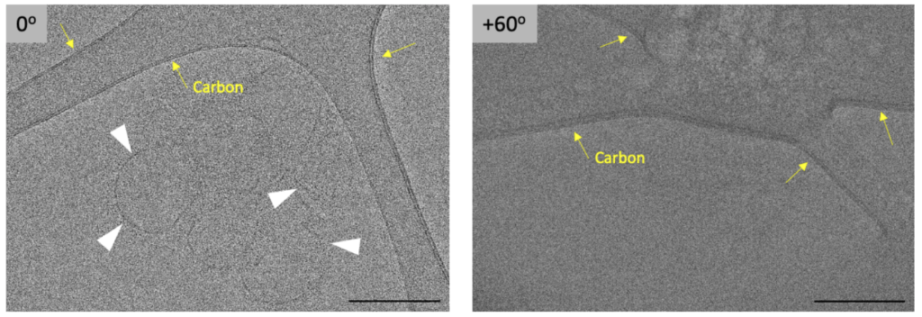
Removing the outlier images is important, because they can otherwise cause severe errors during alignment. Ideally, such images would be removed before alignments are started. However, these ‘bad’ images are often not caught, since large quantities of tilt-series are automatically collected in an imaging session and data processing is moving towards less user intervention and monitoring during refinement steps. These images are then removed when alignments either fail due to severe shifts or the 3D reconstructions appear inadequate.
Low dose exposures per tilt angle accumulate during the course of the tilt-series collection, which leads to increased radiation damage and loss of high-resolution information. This is addressed through dose weighting of each image, which down-weights high frequency information in images collected later in the tilt series that have decayed from radiation damage. As described in the previous chapter, this is why the bidirectional tilt-scheme is preferred for data collection, because the images at low-tilt angles are preserved with the highest resolution. This is especially important for downstream subtomogram averaging steps, which are covered in the next chapter.
All images recorded by transmission electron microscopy are corrupted projections of their true object. The corruptions are a fundamental aspect of TEM imaging that causes an uneven transfer of information content as a function of spatial frequency. This transfer is mathematically represented as a sinusoidal wave known as the contrast transfer function, or CTF.
The CTF is a function of many terms, including electron wavelength (determined by the accelerating voltage of the microscope), the spherical aberration of the microscope (denoted as Cs), and the defocus of the image. Within a cryo-EM dataset, the electron wavelength and Cs terms are constant, but the defocus will vary. Therefore, the most important task in CTF estimation is to determine the true defocus of each image. If the CTF is known for an image, then it can be mathematically applied to restore the authentic version of the image. More information about the CTF, including an interactive module, are available in CryoEM 101.
For cryo-ET imaging, CTF estimations are challenged by relatively low signal-to-noise ratios in each image (e.g., lower doses are used per image in the tilt series) and increased sample thickness (due to sample tilt). Furthermore, tilted images contain a gradient of defocus values throughout the image, because different areas of the image are at different focal heights. It is therefore inappropriate to apply a single defocus value to a micrograph recorded at a tilted angle.
The most common approach to CTF correction of tilted images is to apply the known defocus gradient along strips that are parallel to the tilt axis. Emerging methods also account for variable CTFs due to different focal heights, such as through “3D CTF” correction.
The movies of a tilt series need to be properly aligned to each other to be able to obtain an accurate tomographic reconstruction.
Tilt-series (top) and tomogram (bottom) of vitrified enveloped protein nanocages. The left pair demonstrates how a tomogram would look like if the tilt-series has not been properly aligned yet. Note slight ‘jiggling’ from translations at the tilt-series manifest as blurry features in the tomogram. The membranes of the vesicles are visible but the content, the protein cages are invisible. The edges of the tomogram appear ‘ragged’, since the images are translated and data is absent. The membranes, despite being present, are not traceable throughout the tomogram as a vesicle nor is the bilayer of the membrane visible. On the right, the aligned tilt-series and the corresponding tomogram are shown. The differences to the unaligned version are striking: The membranes are clearly visible, many more vesicles and overall detail appear in the tilt-series, the round shape of the vesicles are clear. Notably, the protein nanocages appear clearly in the vesicles in the tomogram with sufficient contrast to visualize substructures. Data processing was performed using Apprion-Protomo and IsoNet. Data provided by Benjamin Schmitz (University of Utah).
During alignment, variations in translational shifts, rotations, magnifications and sample deformation induced by the electron beam are determined and corrected. These parameters are used to define the 3D projection model for the tomographic reconstruction, such that the quality of tilt-series alignment feeds forward into the quality of the 3D reconstruction. The quality of the 3D reconstruction strongly influences the clarity of the tomogram and the attainable resolution in subtomogram averaging.
The tilt-series alignment procedure is divided into coarse and fine alignment. In coarse alignment, whole-image movements are performed and tilt images with little to no overlap are removed manually. Fine alignment determines the shifts, rotations, magnifications, and sample deformation. Fine alignment of low contrast cryo-ET tilt series can be done using fiducial markers, commonly colloidal gold fiducials added prior to vitrification (see cryoET101 Chapter 2). Fiducial markers give high contrast and are used to align tilt images of a tilt series but often require manual intervention. Alternatively, patch tracking can be used to track movement between tilts (e.g. IMOD), which defines higher contrast features to be tracked instead of gold-fiducials. This is particularly useful for tilt-series generated from cryo-lamella that do not have gold-fiducials. In addition, direct detectors record individual electrons producing high contrast images which increases signal-to-noise ratios, so that image defocus estimation is reasonable making cross-correlation based tilt-series alignments possible. This type of alignment uses cross-correlation of pairwise images and can be combined with projection-matching (Winkler and Taylor 2006, Noble et al. 2015) for more accurate alignments. Fiducialless methods are especially useful for tilt-series generated from cryo-lamella that cannot include fiducial markers.
Recent advances in microscope hardware and data collection software have drastically accelerated the speed of data collection, and the prospect of automated tilt-series alignment with minimal manual intervention is an area of active development. Traditional methods have relied on manual approaches to tilt-series alignments, which can take weeks to months. New automated and faster approaches have been developed and can be extremely helpful for beginners, since important decisions are made by the programs (e.g. AREtomo, Tomo3D). In addition, programs are often adopting ‘all-in-one’ workflows, so users do not have to modify the format of their tilt-series during processing to switch between software packages, which is otherwise time-consuming and challenging (e.g. EMAN2, Scipion).
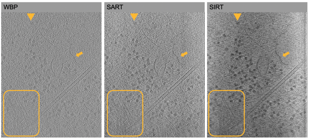
After the tilt-series is aligned, it is time to create a 3D volume from the 2D projections. The most common methods to generate 3D reconstructions are weighted back projection (WBP, e.g. Radermacher, 2006), simultaneous iterative reconstruction (SIRT, e.g. Gilbert, 1972), and simultaneous algebraic reconstruction (SART, Andersen and Kak, 1984).
WBP is the most commonly used method for the 3D reconstruction step. WBP is taking place in Fourier space as are approaches using tilted-direct Fourier inversion borrowed from single particle approaches (Chen et al. 2019). It is not iterative and often used if high-resolution information needs to be retained, e.g. for subtomogram averaging. Each image undergoes Fourier transformation and is placed into a 3D Fourier volume. The tilt angles recorded during data collection are used to determine where to place the fourier plane. In addition, each frequency contribution is weighted to prevent oversampling before back-projecting the volume into real-space, which creates the 3D volume, the tomogram.
In contrast, SIRT and SART are both real-space methods that iteratively refine the 3D reconstruction. This is much more computationally demanding compared to WBP and often requires access to GPU workstations. An initial 3D volume is created and 2D projections are generated from it and compared to the real data. Adjustments are made to minimize errors in the projection matching and reconstruction before the next iteration begins. In SART, the 3D reconstruction is updated one projection at a time, while in SIRT all projections are taken into account before a 3D reconstruction is created. SIRT and SART reconstructions overall are often sharper (higher contrast) and contain less streaking than WBP projections. 3D reconstructions generated by SIRT/SART are ideal for cellular tomography, since they provide more contrast helping downstream annotation and segmentation workflows, while high-resolution information for sub-tomogram averaging is lost.
When looking at 3D reconstructions it is often hard for novices to recognize if the reconstruction is of good quality. The most common issues observed in tomograms and suggestions how to optimize the reconstructions are described in this section.
Drifting is one of the most common problems observed in reconstructions. The sample appears ‘ghostly’, almost as if features are drifting like vapor through the tomographic slices.
The ‘ghostly’ or ‘vapor-like’ appearance is caused by a continuous drift that propagates throughout the tilt-series and can be corrected by removing the drift.
When tilt-series from cryo-lamella are collected, the starting angle is seldom zero degrees. Cryo-lamella are milled at an angle (see Chapters 3), so the first tilt-angle usually needs to be off-set (see Chapter 4). When aligning the tilt-series, the tilt-series off-set needs to be accounted for or the alignment will not be ideal but rather drifting and lower contrast.
Data reconstruction with AREtomo SART. Tomograms of E. coli cryo-lamella prepared using the waffle method. The 3D reconstruction (left) has not been corrected for the tilt-offset and is blurry. In the right 3D reconstruction the tilt-offset of 20 degrees has been corrected for and has markedly improved. No drift and contrast is enhanced. Data provided by Jake Johnston (Columbia University, NYSBC). Download video here (left) and here (right).
The thickness selected for tilt-series alignment and reconstruction is another important parameter with impact on alignment and reconstruction quality. If the sample thickness is estimated too large, there will be a substantial amount of noise to be aligned, impairing proper alignment. Similarly, if parts of the tilt-series won’t be included in the aligned because the thickness is chosen too narrow, the tomogram quality will be impaired since parts of the tilt-series will not have been aligned. During alignment and refinement runs different thicknesses can be chosen to optimize the 3D reconstruction. In addition, the milling angle for cryo-lamella needs to be taken into account to further improve the reconstruction.
Reconstructions (AREtomo SART) of cryo-lamella of E. coli prepared using the waffle method. Left a thickness of 1500 nm was used. Note the drift, the ‘wiggling’ ribosomes (dark spheres) and ‘wobbly’ membranes. In the center video, a thickness of 2000 nm was used which improved the reconstructions, however, there is still movement as if the ribosomes float. When the milling angle of 20 degrees is corrected for during alignment and reconstruction, the E. coli membranes stay in place and the ribosomes stop ‘wiggling’ (right video). Also, contrast is improved. Data provided by Jake Johnston (Columbia University, NYSBC). Download videos here (top left), here (top right), and here (bottom left).
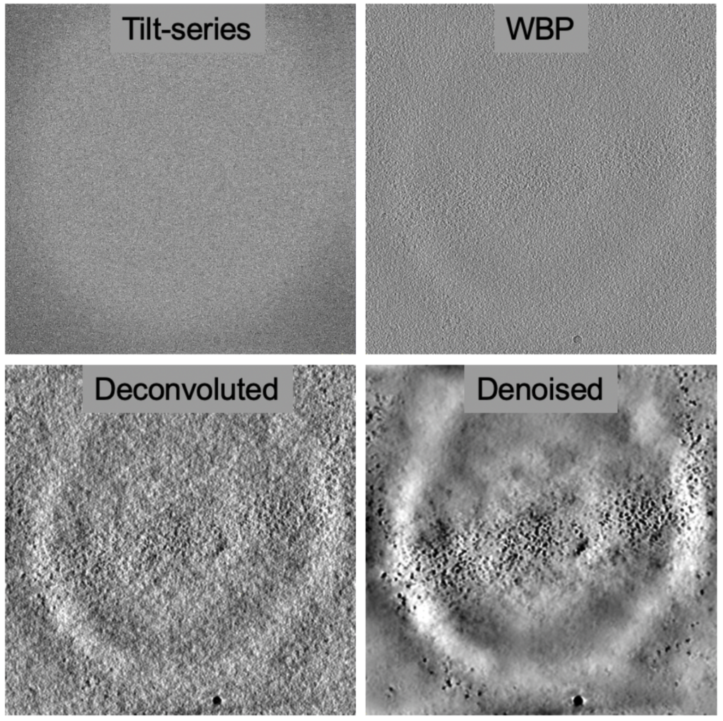
One of the challenges of cryo-ET is low signal-to-noise-ratios leading to low contrast in the 3D reconstructions. The field has been grappling with this problem for a while and deconvolution approaches with the goal to reduce the point-spread-function and denoising approaches helping to create a featureless background have been both useful to enhance contrast. Deconvolution steps have become part of software suites, e.g. AREtomo2 and Warp, which help by providing more contrast for the alignment and reconstruction.
Artificial Intelligence (AI) image processing approaches, particularly convoluted neural-networks, are being adopted for cryo-ET workflows to help overcome low signal-to-noise ratios and missing wedges. These networks are particularly helpful when they are pre-trained to be used ‘right out of the box’. The goal of “denoising” approaches is to improve image contrast to ‘nullify’ the noise originating from low electron exposures, so that details can stand out against the background (e.g. Topaz-Denoise) and more elusive details hidden in the ‘noise’ can be recognized, picked and evaluated.
One of the most fundamental limitations in cryo-ET is the loss of data due to missing wedge artifacts (CryoET 101, Chapter 4), which leads to anisotropic data. This manifests in ‘smearing’ of the map in one direction due to the missing information. Subtomogram averaging can overcome missing wedge artifacts because the averaging of multiple particles in different views will fill in the missing wedge from each particle. However, if cellular structures are of interest, averaging is not an option.
The software package IsoNet has made progress towards filling in the missing wedge using a neural network without the need of STA. The deep-learning based software uses information obtained from within the tomogram to fill in the missing information. It currently performs best on cellular tomograms of pixel sizes of 10 Å but can provide structural information up to 30 Å, which can be very helpful for segmentation. The signal-to-noise ratios are improved owing to less anisotropic data.
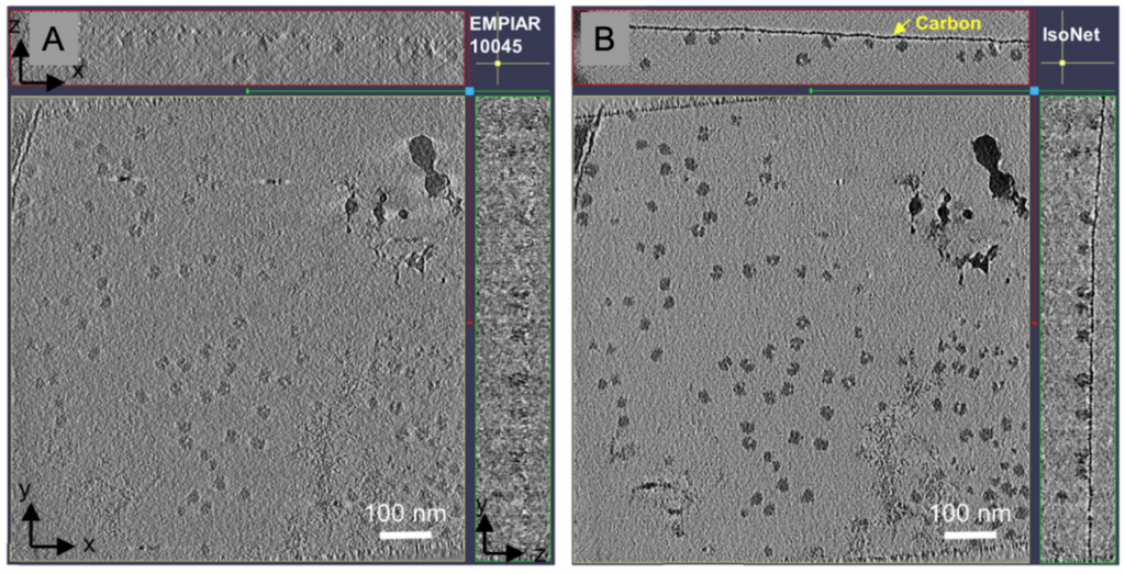
Both, denoising software packages and the IsoNet suite, aid analysis of high-resolution cellular tomograms – or tomograms of purified samples – since they help to discern the particles in the 3D reconstruction, which might be otherwise missed. The particles can then be selected and annotated or further processed using STA.
Data processing as a whole is not a one-and-done process. Tilt-series alignment and 3D reconstruction steps are rather iterative, especially, since the quality of the alignment can be best evaluated as a 3D reconstruction, where the quality becomes apparent. You have now learned to be cognisant of the common strategies during processing, can decide when to use WBP vs. SIRT/SART for reconstructions, are aware of common pitfalls and can judge if the alignments are adequate and the 3D reconstruction can be considered “finished”. Please see excellent reviews, e.g. Pyle et al. 2021, for more details and great starting points for selection of appropriate software, and #teamtomo.org for step-by-step processing examples. In addition, most software suites have excellent github pages with instructions or tutorials available.
Please use the processing program suites listed in the table as a starting point for tilt-series alignment and reconstruction.
| Program suite | Download information |
| Warp | http://www.warpem.com/warp/# |
| EMAN2 | https://github.com/cryoem/eman2 |
| TomoBear | https://github.com/KudryashevLab/TomoBEAR |
| Tomo3D | https://sites.google.com/site/3demimageprocessing/tomo3d |
| AREtomo2 | https://github.com/czimaginginstitute/AreTomo2 |
| ScipionTomo | Released upon request. https://doi.org/10.1016/j.jsb.2022.107872 |
| IMOD | https://bio3d.colorado.edu/imod/ |
| Dynamo | https://www.dynamo-em.org//w/index.php?title=Main_Page |
| Appion-Protomo | https://github.com/nysbc/appion-protomo |
| IsoNet | https://github.com/IsoNet-cryoET/IsoNet |
| Topaz-Denoise | https://github.com/tbepler/topaz |
You are ready for the next steps of either subtomogram averaging or annotation and segmentation of your tomogram to extract the information within and reveal exciting biological findings. Please move on to the next chapter to learn more about these final steps.
© Copyright 2024