
In this final chapter of CryoEM 101, we will cover the principles of how cryo-EM images are used to generate 3D reconstructions. The typical data processing workflow entails the following steps, each of which are discussed in greater detail below:
There are many software options available to carry out these tasks, but this chapter will not describe details of specific programs or packages. Rather, the major objective of this chapter is to teach the general principles of how each step of image processing works and the guidelines to getting the most out of your data.
The first step in processing cryo-EM data is to correct for the movement of particles that occurs when specimens are exposed to the electron beam. This phenomenon is referred to as ‘beam-induced motion’ and has been well characterized since direct detector technology was introduced to the field. The high sensitivity and fast frame rate enabled by direct detectors allow cryo-EM data to be recorded in the form of movies. Modern algorithms have been developed to accurately align individual movie frames against each other. This realignment corrects for beam-induced motion, after which the re-aligned frames are then summed into a single, de-blurred micrograph.
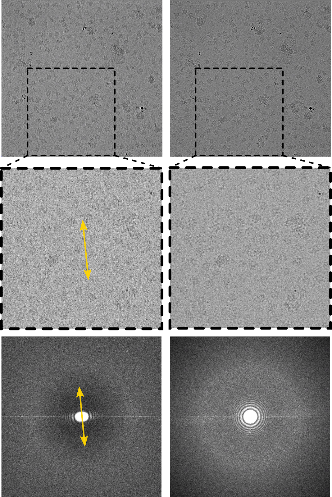
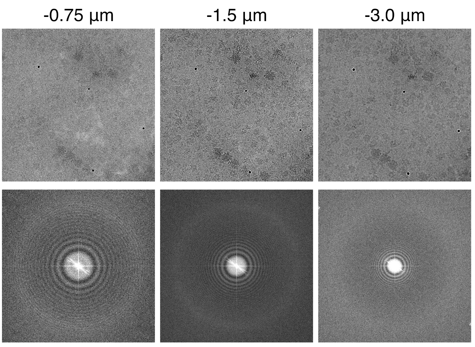
The ability to correct for the effects of beam-induced motion is among the greatest breakthroughs in cryo-EM. Images recorded using traditional detectors, such as film and CCD cameras, were often blurry because particle movement during image acquisition amounted to taking a picture of a moving target. As shown in the figure below, the effects of such motion are especially noticeable by the directional loss of Thon rings in the power spectrum of the image. Correcting for the motion enables the high-resolution content to be recovered.
Before ……………………………. After
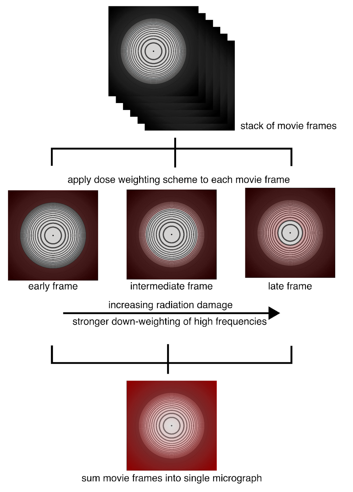
The electron beam used in cryo-EM imaging damages biological material during the course of exposure. Cryo-EM movie frames therefore accumulate an increasing amount of electron dose. The earliest frames contain the most pristine information and relatively low radiation damage, but the low amount of electrons in these frames produce limited contrast in the images. The accumulation of electrons led to higher contrast images in later frames, but high-resolution information is quickly degraded by radiation damage. Modern algorithms employ a dose weighting, or exposure filtering, scheme that downweights high-resolution content from movie frames as a function of their accumulated doses. Consequently, early frames retain their high-resolution content while the information in later frames is limited to low-resolution content. This dose weighting, or exposure filtering, scheme allows the best information to be used for downstream image processing by excluding radiation damaged components from the summed micrographs.
All images recorded by transmission electron microscopy are corrupted projections of their true object. The corruptions are a fundamental aspect of TEM imaging that causes an uneven transfer of information content as a function of spatial frequency. This transfer is mathematically represented as a sinusoidal wave known as the contrast transfer function, or CTF. In standard TEM imaging, the CTF starts near zero at low spatial frequencies and oscillates between positive and negative maxima (corresponding to positive and negative contrast transfer, respectively) and zero-crossings are indicative of frequencies that contain zero information. The CTF is further modified by envelope functions as a result of spatial and temporal incoherence by the electron beam, which dampens the CTF at high spatial frequencies.
The purpose of estimating CTF parameters is to enable the computational correction of the CTF to each image. The CTF is a function of many terms, including electron wavelength (determined by the accelerating voltage of the microscope), the spherical aberration of the microscope (denoted as Cs), and the defocus of the image. Within a cryo-EM dataset, the electron wavelength and Cs terms are constant, but the defocus will vary. Therefore, the most important task in CTF estimation is to determine the true defocus of each image. If the CTF is known for an image, then it can be mathematically applied to restore the authentic version of the image. Note that zero-crossings in the CTF cannot be recovered as there is a complete loss of contrast transfer. This concern is readily mitigated because the missing information in one micrograph will be covered by a different CTF in another micrograph that was recorded at a different defocus.
Oscillations within the CTF are easily seen by visualizing the power spectrum of cryo-EM images. High quality images will show a pattern of concentric rings that represent the alternation of high and low contrast transfer as a function of spatial frequency. The origin of the power spectrum is at the center of the image and represents regions of low spatial frequencies. The edge of the power spectrum represents the maximum spatial frequency defined by 2x the pixel size, or the Shannon-Nyquist limit. (As described in the previous chapter, the pixel size and Nyquist limit are directly related to the magnification used during imaging.)
CTF modeling is also an effective way to assess micrograph quality in an objective manner. Thon rings are radially averaged to generate a 1-dimensional plot of the CTF as a function of spatial frequency. CTF estimation programs fit the observed CTF to a theoretical model, and the quality of fit is assessed by their cross-correlation. The fitting also reports the resolution in which the data no longer fits the model. Together, the cross-correlation and resolution limit of CTF fitting are useful metrics to exclude poor micrographs out of the dataset.
The following interactive module provides a simple interface to visualize the 1D representation of the CTF. Adjust various parameters within the module to test how they influence the shape of the CTF. Note how the CTF is modified by relative defocus: high defocus images are generally disfavored because of their frequent zero-crossings, but their initial maxima at low spatial frequencies produce high-contrast images; low defocus images contain better preserved information (due to fewer zero-crossings), but their content may be invisible to the eye.
More information about CTF principles and theory are available in these video lectures:
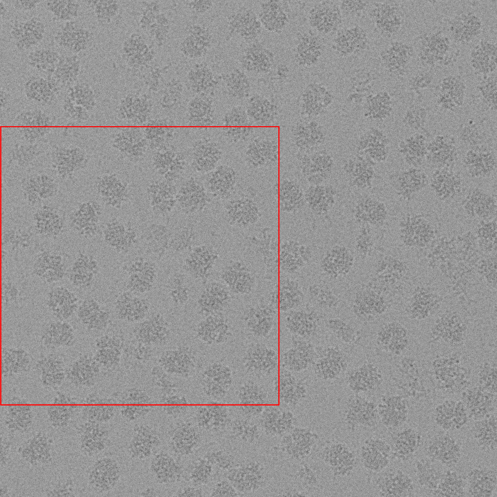
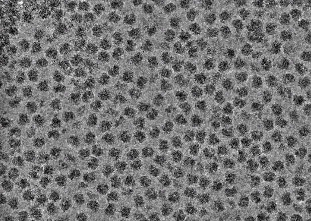
The next stage of data processing is to identify and extract individual particle images from the motion-corrected micrographs. Many approaches are available to pick particles, from fully manual to fully automated approaches. A semi-automated approach that uses both manual and automated particle selection is a highly recommended way to optimize between time and accuracy. In this approach, a few hundred particles are manually selected from a few representative micrographs that cover the defocus range of the dataset. These particles are used to compute low-resolution 2D class averages (discussed more below), and these classes serve as templates for automatic particle picking for the entire dataset. Another common method for particle picking is to simply use a gaussian blob of a defined radius range. Both of these approaches are commonly used and represent ways in which a large number of particles can be selected in an efficient and reasonably accurate manner. It is acceptable to err on the side of over-picking to maximize the number of particles extracted from each micrograph because downstream methods are effective to exclude empty or junk picks.
Regardless of the method used for particle picking, the most important consideration is that the selected particles are visible by eye. One useful tool to enhance particle contrast is to apply a low-pass filter when particle picks are being evaluated. A low-pass filter excludes all high-resolution frequencies beyond the defined cutoff (e.g., a 10 Å filter will remove all signal < 10 Å from the image). Use the following interactive to see how the visual qualities of a cryo-EM image are affected by low-pass filtering. Note that such filters are only used for visualization purposes: the extracted particles will not have the filter applied to them.
After particles have been selected, they are then extracted from the micrographs to generate a particle stack. Particles are extracted with square dimensions and should include a generous amount of solvent space. As a general rule of thumb, box sizes should be approximately 50% larger than the longest view of the particle (e.g., a particle with a ~200 Å diameter at its longest view should use a box size that covers ~300 Å). The reasons for this requirement are twofold: first, there needs to be sufficient solvent area for downstream processing steps to distinguish the particle from noise; second, the delocalization effects associated with the CTF may extend beyond the visible components of each particle image. For practical reasons, box sizes also needn’t be overly large as it would add unnecessary computation burden to downstream image processing steps.
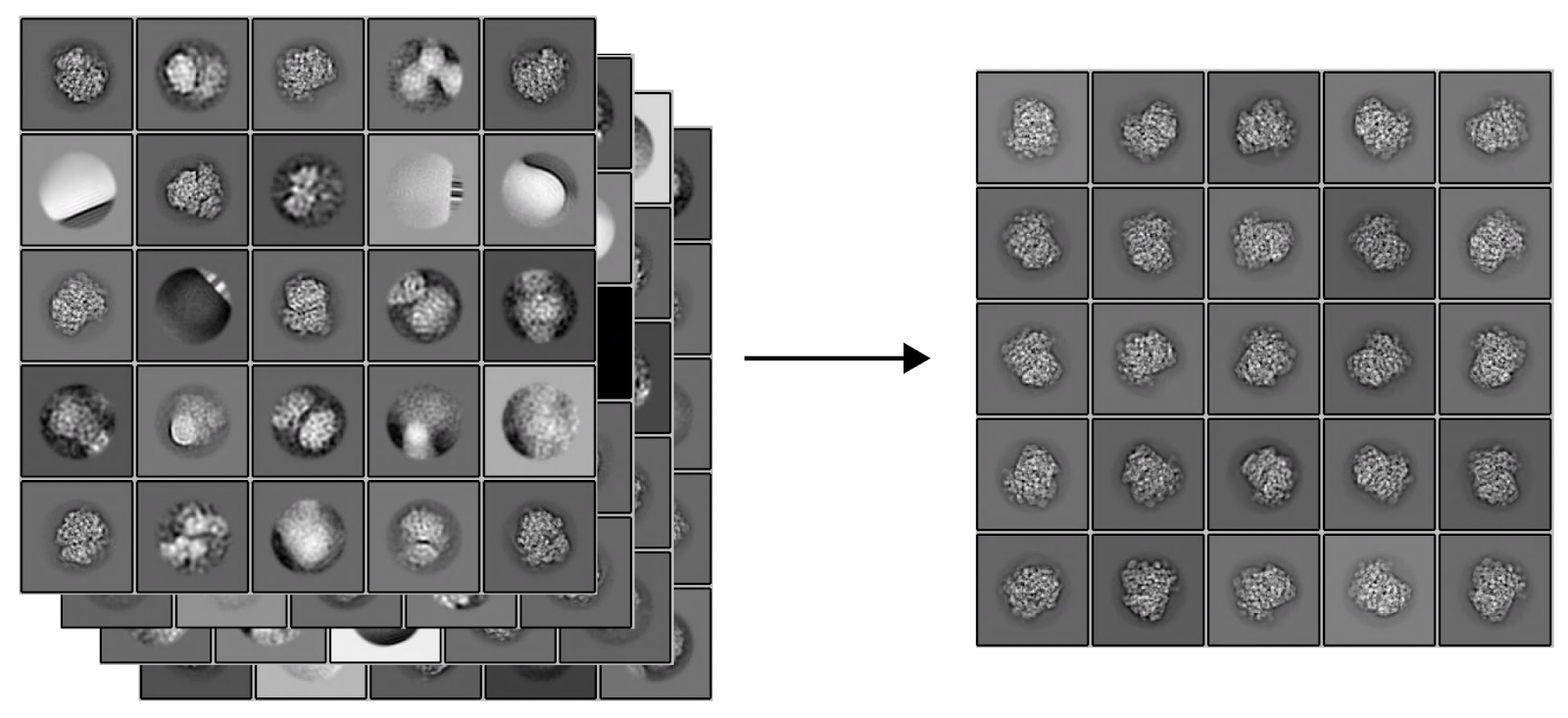
After picking particles, the stack of extracted images are used for 2D classification. The concept behind 2D classification is simple: particles within a dataset are compared against each other and similar particles are clustered into groups, or classes. The classification process accounts for differences in x, y translation, in-plane rotation, and CTFs, and resulting “class averages” reveal enhanced details because of their increased signal-to-noise ratios compared to raw images. In other words, consistent features among particles are reinforced and the effects of noise are averaged out.
Although 2D classification is not strictly a necessary step along the structure determination pipeline, this procedure can provide invaluable insights. Importantly, 2D classification is often the definitive step along the cryo-EM workflow where orientation bias and structural heterogeneity is revealed. If there are only a limited number of distinguishable 2D classes, this is often a clear indicator that the dataset lacks a broad distribution of unique views. If the 2D classes lack well-resolved features, then there may be issues with the imaging or sample quality, or that the particle itself is poorly averageable.
In addition to confirming the relative quality of particle images, 2D classification is also a straightforward way to curate the stack of extracted particles. Specifically, particles sorted into well-resolved classes are separated into a refined stack from other particles that are sorted into poorly resolved or “junk” classes. It is normal at this stage to throw out a substantial number of particles depending on how accurate particle picking was performed. Multiple rounds of 2D classification can be performed to refine the quality of classes and to increase confidence that only the best particles are used for downstream steps. The refined stack is then used as the input for 3D classification and reconstruction.
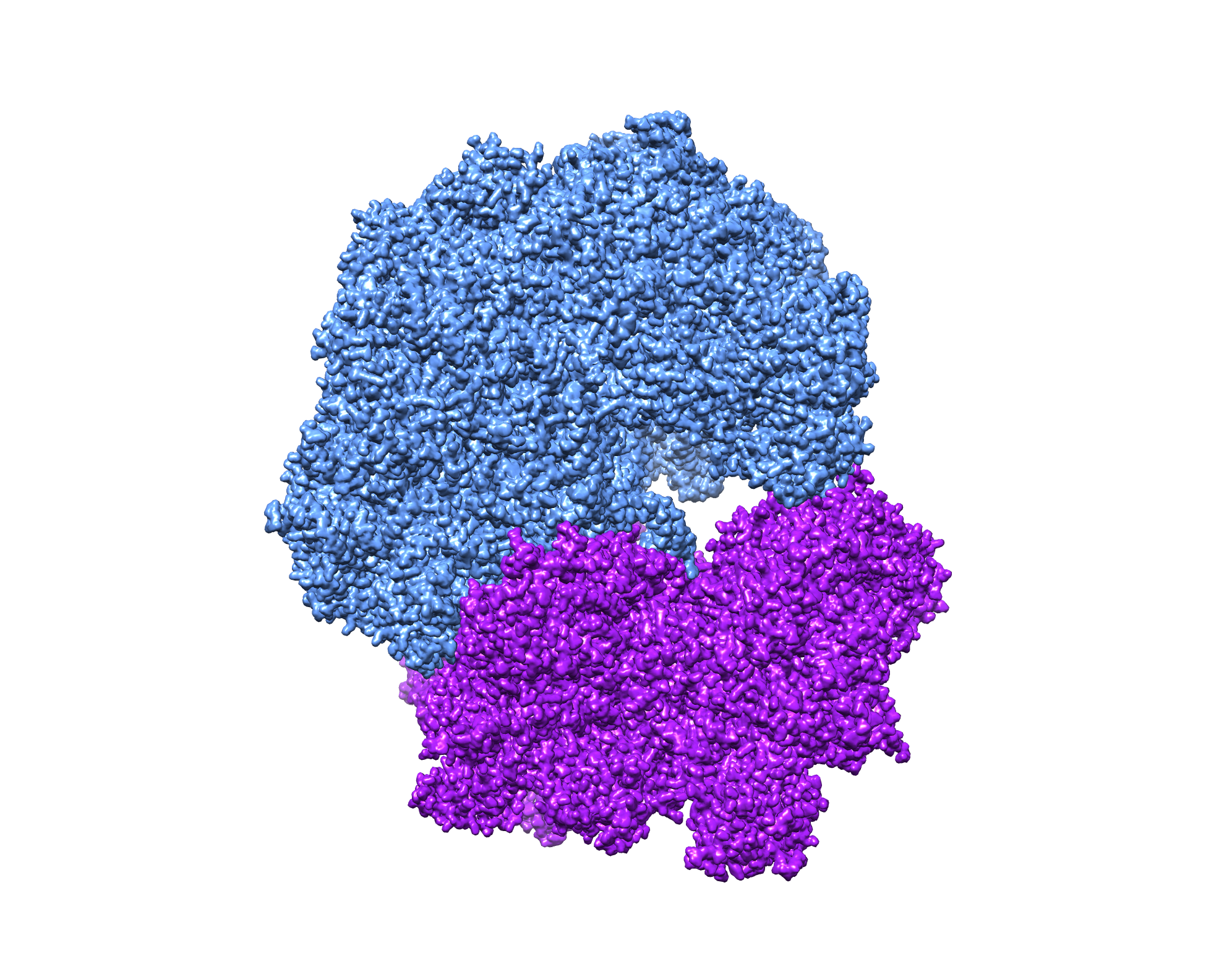
Particle images represent 2D projections of the original 3D object. The challenge underlying 3D reconstruction is that the relative orientations of the particle images are unknown and their determination is generally the rate-limiting step in the reconstruction process. The most common way to determine particle orientation is through “projection matching” algorithms in which cryo-EM images are compared against projections of a reference 3D model. Reference models are generally derived from related structures or can be generated with ab initio methods. Importantly, the reference models used are ideally low-resolution to minimize unintended effects of model bias. After relative orientations are assigned, each particle image is back-projected into a new 3D reconstruction.
3D reconstruction is an iterative process in which each new reconstruction serves as the reference model for the next cycle. Each new cycle strives to improve the accuracy of orientation assignments, and more accurate orientations will produce higher resolution maps. After several cycles, the reconstruction job reaches a point where successive iterations do not lead to significant changes in orientation assignments and the reconstruction resolution. The job is described to have ‘converged’ and completes upon the generation of the final map.
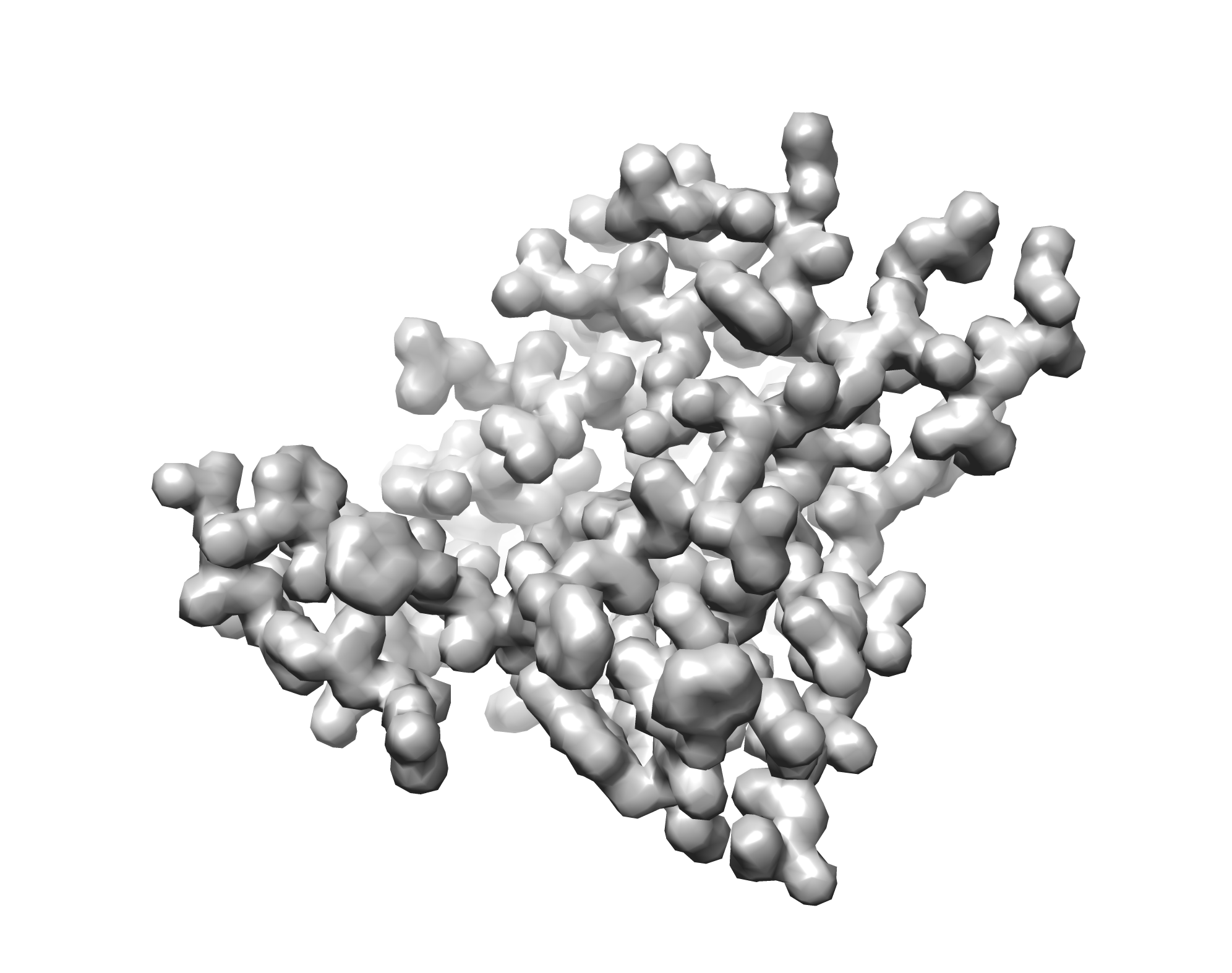
The following interactive panel provides examples of ribosome maps filtered to different resolutions. Typical reconstruction jobs start with a low-resolution reference (filtered to ~40-60 Å). Despite the blobby, featureless nature of such references, they provide sufficient information for assigning initial orientations. Orientation assignments are refined as the job progresses and will produce higher resolution reconstructions with each successive iteration.
As with 2D classification, particles can also be classified in 3D to sort them among different structural states. This type of 3D classification is especially useful to distinguish among particles that exhibit compositional and conformational heterogeneity.
Leading reconstruction algorithms use a so-called “gold standard” approach in which datasets are divided into two halves and each half is processed independently. The reconstructions computed from each half-dataset, known as ‘half maps’, are correlated against each other after each iteration to estimate resolution. These correlations are referred to as “Fourier Shell Correlations,” or FSCs, and are calculated by cross-correlating the half maps as a function of spatial frequency (or Fourier shells). The resolution cutoff at which the FSC crosses the 0.143 threshold is the most commonly used criterion to report the nominal resolution of cryo-EM reconstructions*. Half maps are filtered to the resolution at the FSC=0.143 threshold and then used as the new model for the next iteration of 3D reconstruction. After the job converges, the half maps are summed together and then filtered to the final resolution at the FSC=0.143 cutoff to output the final map. Although each job reports a final resolution, it is important to emphasize that assigning a single nominal resolution to a reconstruction is often an insufficient (and sometimes inaccurate!) way to assess map quality because a reconstruction can comprise a mixture of well resolved and poorly ordered components.
* The FSC=0.143 threshold is based on an X-ray crystallography standard for map interpretability. More details about its origins are described in the paper Rosenthal & Henderson. J. Mol. Biol. (2003).
The final step to cryo-EM data processing is to validate the quality of your results. In other words, how do you know that your reconstruction is reliable? Several quality control metrics should be used to support the interpretation of 3D reconstructions.
Is your reported resolution consistent with the visualization of expected features at that resolution? The following interactive module shows the quality of density maps at different resolutions. At 2 Å, the definition of the protein backbone and side chains are unambiguous. At 3 Å, most side chains can be modeled. At 4 Å, the protein backbone can be traced and bulky side chains are present as bumps. Importantly, the pitch of alpha helices and separation of beta strands are preserved at this resolution. At 5-8 Å, we begin to lose separation of beta strands and the tracing of the peptide backbone is unreliable. Alpha helices are visible as rod-shaped densities. Beyond 8 Å, there is insufficient resolution for reliable modeling and structural interpretation is limited to rigid-body fitting of other models.
Other validation methods to be posted soon.

© Copyright 2024