

Your sample and grids have been optimized and are ready for cryo-EM data collection. What happens next? In many cases, your grids will be handed or shipped off to a cryo-EM facility where trained experts will load your specimens into the microscope. This chapter introduces the major steps of how data collection works and the decisions that users have to make in order to get the most out of their data.
If you have access to high-end data collection instrumentation at your own institution, then you may want to skip to the next section. Recent efforts to democratize cryo-EM access in the United States have been pushed forward by the establishment of NIH-funded national centers. The mission of these centers is to provide training to cryo-EM newcomers and free-of-charge access. More information about these facilities and how to access them are provided at their websites:
The grids used for cryo-EM data collection are handled exactly the same way as with cryo-EM screening. As described in the previous chapter, grids that are inserted into modern, high-end instrumentation are assembled into cartridges and loaded into a multi-grid cassette. The cassette is loaded into the microscope and the operator selects the grid to load onto the stage. Before starting data collection, it is good practice for the operator to check that the microscope is behaving optimally. These procedures are typically done on a non-biological calibration specimen to test beam alignment and resolution limits. If the tests meet performance standards, then the calibration grid is exchanged for the cryo-EM specimen, and the session proceeds with screening as described in the previous chapter and data collection.
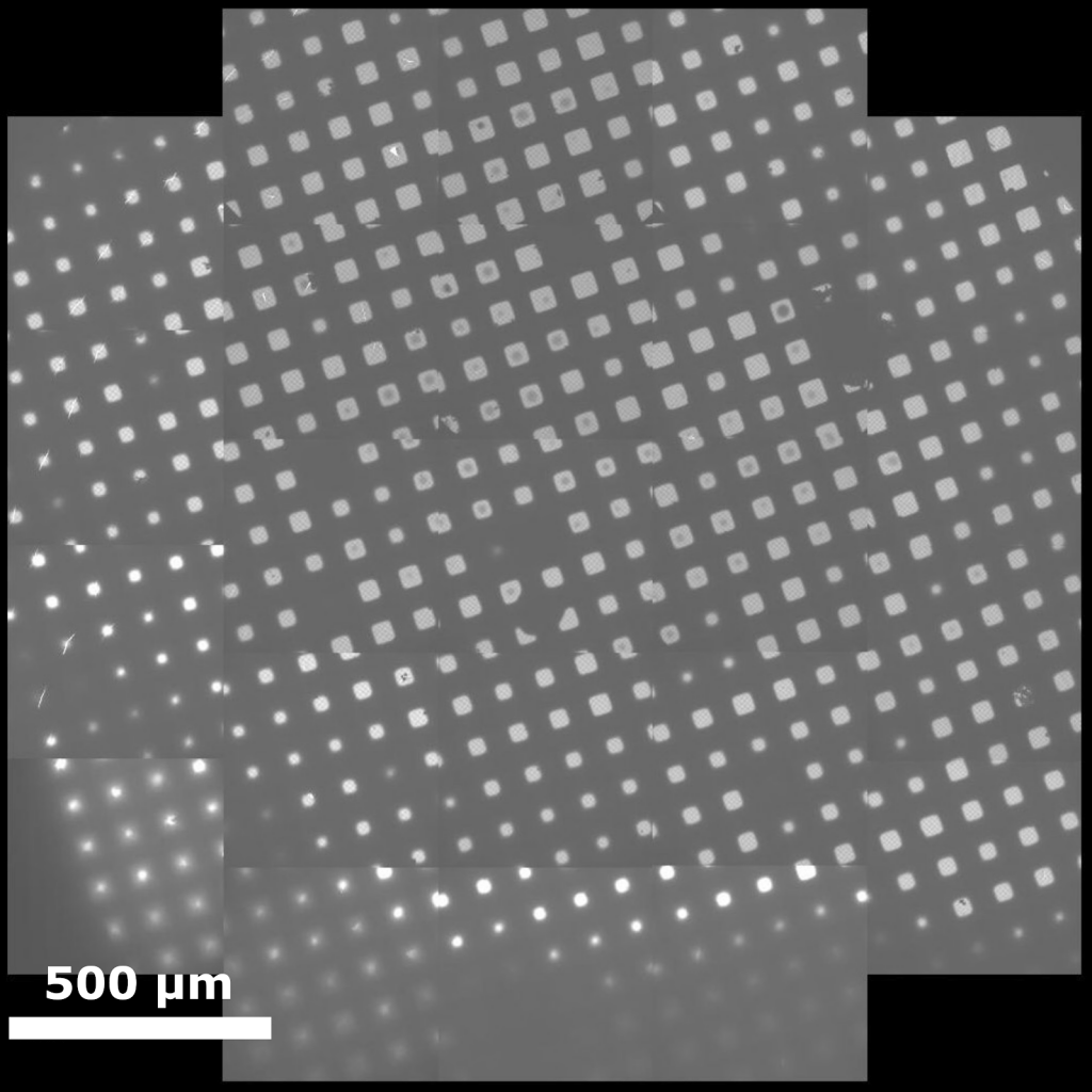
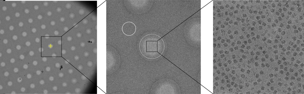
The data collection session typically begins by recording an ‘atlas’, which maps out the explorable areas throughout the grid. The atlas is generated by recording several overlapping low-magnification images, which become stitched together to give a comprehensive view of the grid. Grid atlases serve as convenient references for users to identify the most promising areas of the grid for data collection and are used by data collection software to navigate to specific grid squares. After the user has identified squares of interest, a panoramic view of each square is recorded in a similar way in which the atlas was acquired. Ideally, each grid square contains dozens to hundreds of individual holes that are suitable for data acquisition. Thousands of holes are typically recorded over the duration of a standard data collection session.
The data collection workflow uses a so-called “low dose” approach that cycles between three modes: search, focus, and record. The “search” mode step centers the microscope stage over an imaging area at low magnification. After the area is centered, a focusing step is performed to set the target defocus of the image. The focusing is performed at a position away from the hole in order to protect the particles from radiation damage. After the defocus is set, a multi-second exposure is recorded over the target hole in the form of a short movie. Each movie contains several frames that are processed and summed into a single image. The search-focus-record process is then repeated for the next hole until all target holes have been recorded.
Even if you are not operating the microscope, you will be expected to provide input on a number of parameters that will influence various aspects of your data collection session. These parameters often involve certain trade-offs, such as maximizing resolution versus throughput or balancing between low-resolution and high-resolution content. A few of the most common and important user decisions are described below:
The magnification used for data collection dictates the pixel size of the image and therefore the physical resolution limit. An optimal magnification will strike a balance between the number of particles per field-of-view and the achievable resolution. High magnifications will produce images with fine pixel sizes, but will reduce the number of particles per field-of-view. Larger box sizes will be needed to extract individual particle images, which may pose a computational burden and complicate downstream image processing steps. On the other hand, low magnifications will produce images with coarse pixel sizes and limit the achievable resolution.
The pixel size is defined as the physical distance represented by each pixel. Use this interactive module to explore the relationship between pixels and physical distances from this cryo-EM image of ribosomes. Image acquired with a K2 direct detector, which outputs 3710×3838 pixel images. Example shown here truncated to 3710×3710 for clarity.
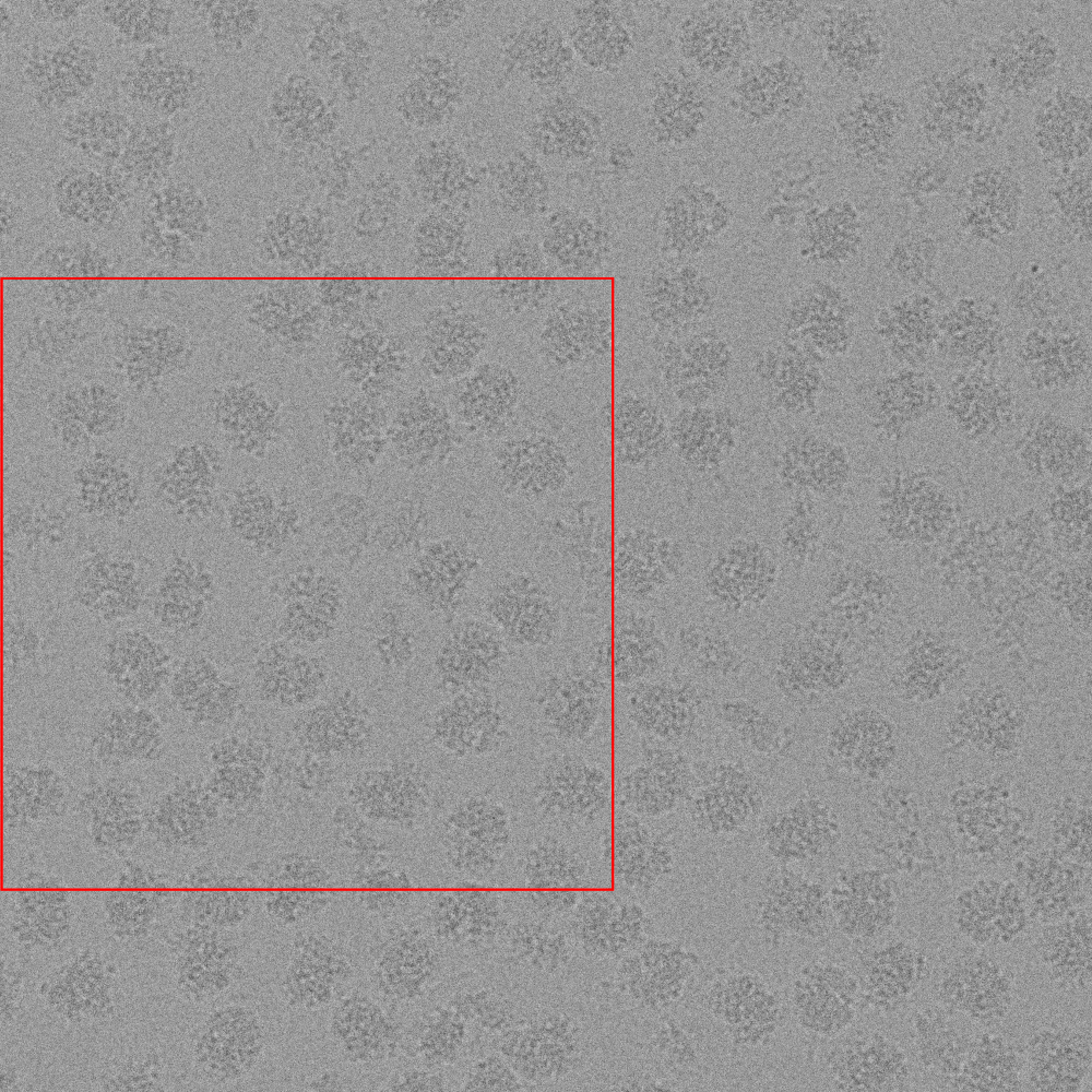
The “Nyquist limit” is a term commonly used among cryo-EM practitioners to refer to the maximal achievable resolution from a dataset. The term is derived from the “Nyquist-Shannon sampling theorem”, which in the context of cryo-EM imaging refers to the maximum theoretical resolution imposed by the pixel size. The Nyquist limit simply refers to twice the pixel size, e.g. images recorded at 1.0 Å per pixel have a physical limit of achieving 2.0 Å resolution. In practice, achievable resolutions are generally considered to fall short of Nyquist due to the dampening of high-resolution signal from microscope and camera properties.
Phase contrast in cryo-EM images is generated by applying a mild amount of defocus during image acquisition. An optimal defocus range will balance between retaining high-resolution information and generating sufficient contrast to identify particle images. If the micrograph is too close to focus, then particles may be invisible. If the micrograph is too far from focus, then there will be an attenuation of high-resolution information. Smaller particles may require higher defocus settings to generate sufficient contrast. Cryo-EM datasets are typically collected with a minimum defocus of -0.5 to -1.0 μm and a maximum defocus around -2.0 μm, though higher defocus settings are warranted if the particles are difficult to see. A range of defocus settings is used so that the dataset contains maximum information across Fourier space. More discussion on the relationship between defocus and resolution will be available in the Contrast Transfer Function section of Chapter 5.
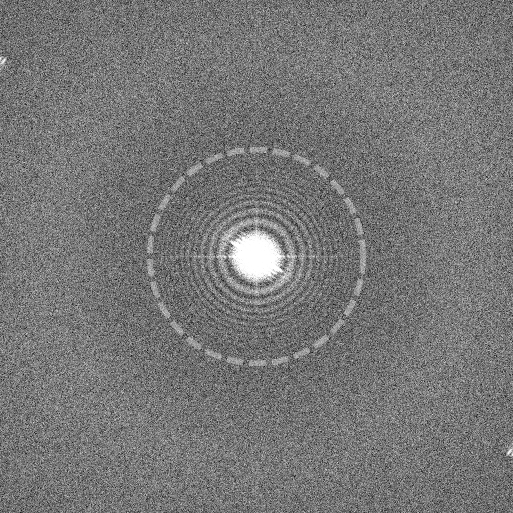
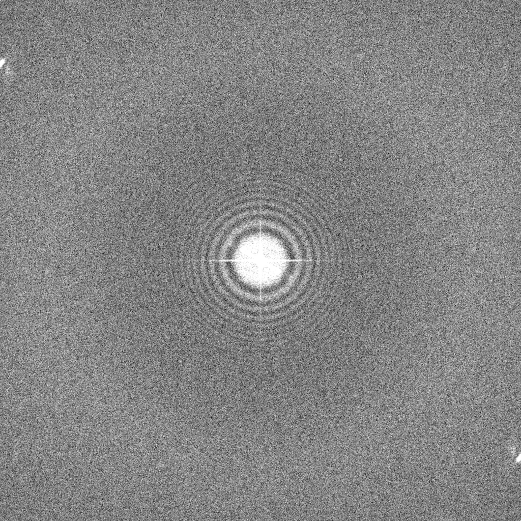
The following image gallery shows examples of cryo-EM images recorded over the same field-of-view at different defocus values using a Titan Krios (300 kV) and K2 detector. The power spectrum is shown on the right of the cryo-EM micrograph, which shows patterns known as Thon rings. Thon rings provide information about the information content of the image as a function of spatial frequency, or resolution. The white rings represent spatial frequencies that contain information, while the gaps between rings and otherwise dark areas represent spatial frequencies with low or zero information.
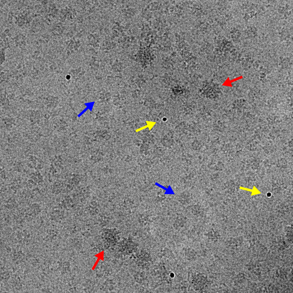
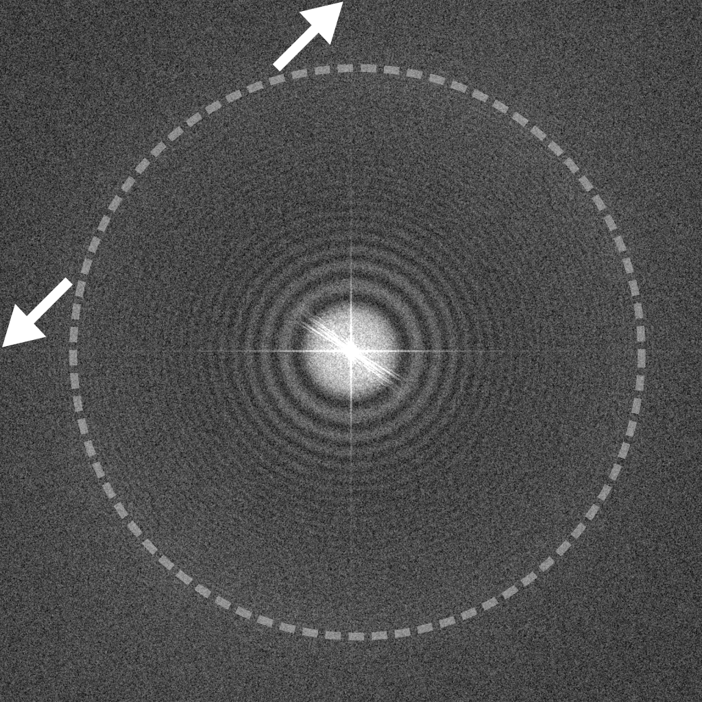
Image recorded at -1.5 μm underfocus (left) contains a mixture of particle types, including ribosomes (red), smaller protein complexes (blue), and gold nanoparticles (yellow). This image shows a good balance between particle contrast and extension of Thon rings to high spatial frequencies (right, dashed circle). The edges of the power spectrum indicate the Nyquist limit (white arrows).

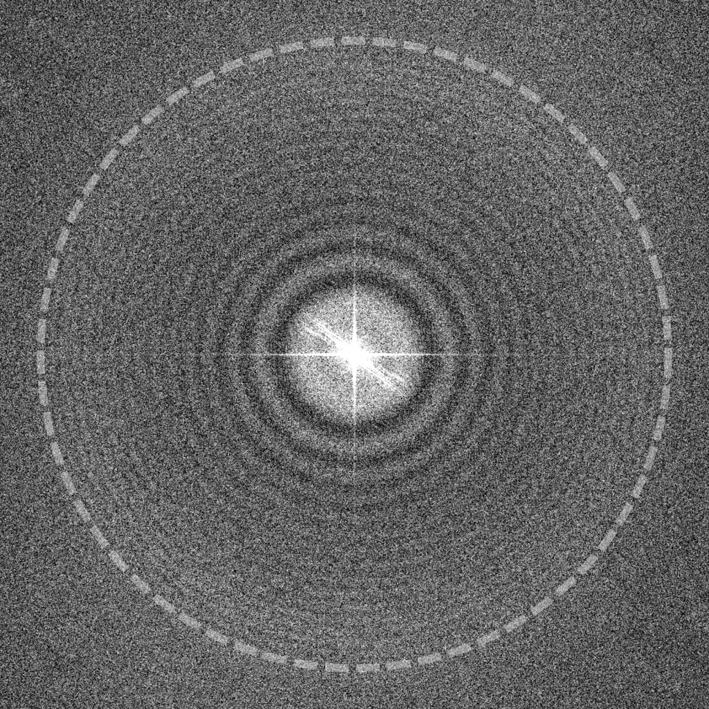
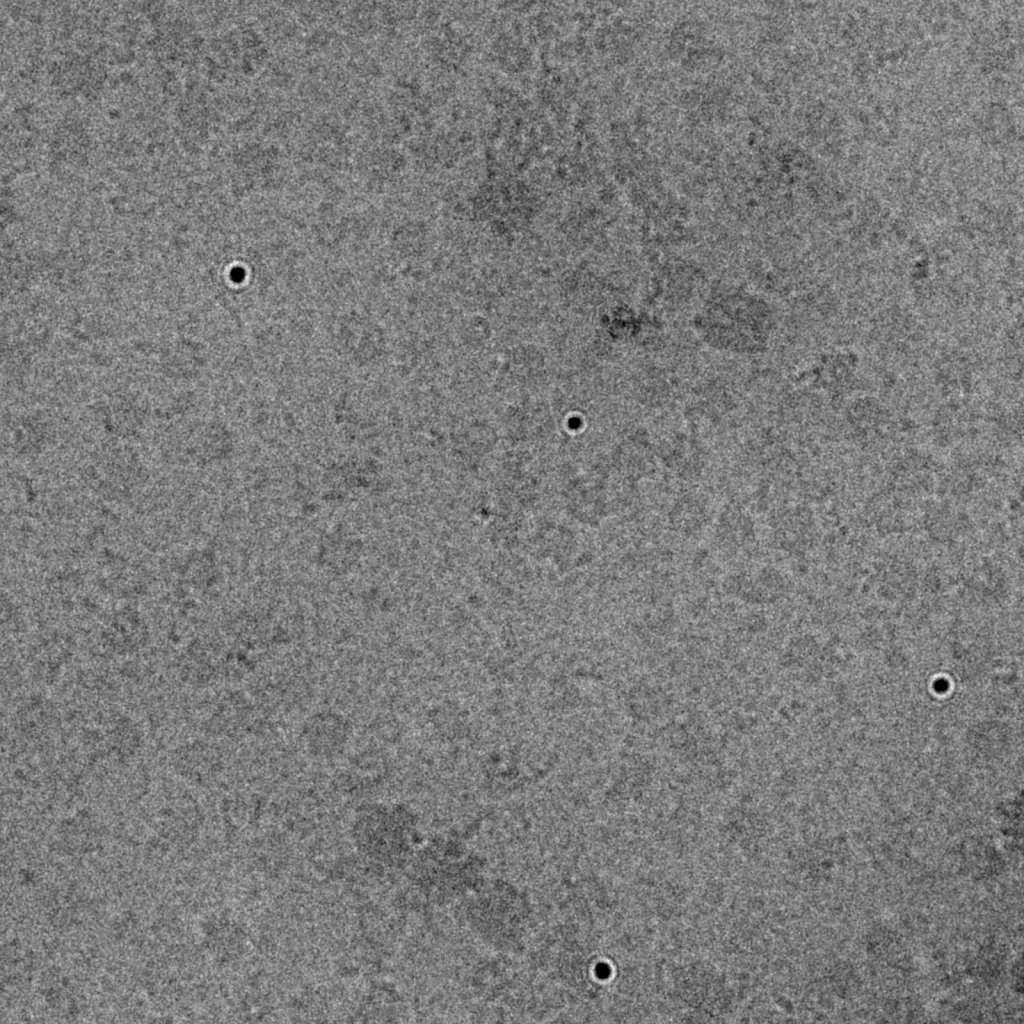
Image recorded at -0.75 μm underfocus (left). Note that Thon rings extend farther out in resolution towards the Nyquist limit (right, dashed circle), but particle contrast is greatly reduced. In this case, the larger ribosome particles (red) are easier to see than the smaller protein particles (yellow) due to their size difference and the rich phosphate content in ribosomes that provide scattering electrons more strongly. Being able to confidently identify particles will be of critical importance in downstream data processing.
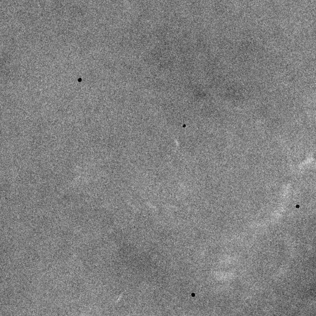
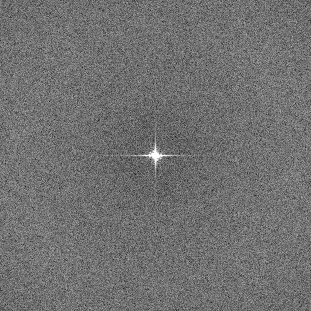
Image recorded at focus. Particles contain minimal contrast and there are no Thon rings. Such images are unusable for data analysis because particles are invisible and cannot be extracted in a reliable manner. The gold nanoparticles are easily observable due to their high electron scattering potential.
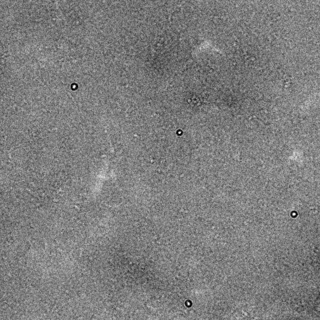
Why not simply apply higher defocus to images if they provide rich contrast, such as this one recorded at -3.0 μm underfocus (left)? Unfortunately, higher defocus settings lead to a strong attenuation of high resolution signal. As shown on the right, the Thon rings fade at earlier resolutions compared to the images recorded at -1.5 and -0.75 μm underfocus (dashed circle). Highly defocused images also produce strong delocalization fringe effects that are most easily seen in this image at the edge of the gold nanoparticles. Despite these drawbacks, higher defocus values may be advantageous for data collection if particles are difficult to see (e.g., for small particles) and if pushing high resolution is not an immediate priority.
What about overfocusing images? Here, an image recorded at +3.0 μm overfocus shows an interesting phenomenon that we encountered in Chapter 1 where contrast becomes inverted at low spatial frequencies and produces a strong dark-light-dark alternating fringe effect that is most obvious in the gold nanoparticles. Recording images with overfocused settings is not recommended because the CTF estimations at these low spatial frequencies is error-prone.
The electron source represents a double-edged sword for cryo-EM imaging: the very source used to generate images causes substantial damage to the particles as they are imaged. An optimal amount of electron exposure, or dose, will balance between generating sufficient signal per movie frame and minimizing radiation damage during the course of electron beam exposure. If the dose is too low, then there may be insufficient data in individual movie frames for motion correction. In contrast, high doses may lead to excessive radiation damage. Nowadays, excessive doses are routinely mitigated by applying a dose weighting, or exposure filtering, algorithm during motion correction procedures. This algorithm essentially down-weights the radiation-damaged components that accumulate in later movie frames while retaining their low-resolution components that contribute to image contrast. Typical electron doses range from 40-60 electrons per Å2, but effective exposure filtering can be performed for even higher doses. The principles of motion correction and dose weighting will be discussed in greater detail in Chapter 5.
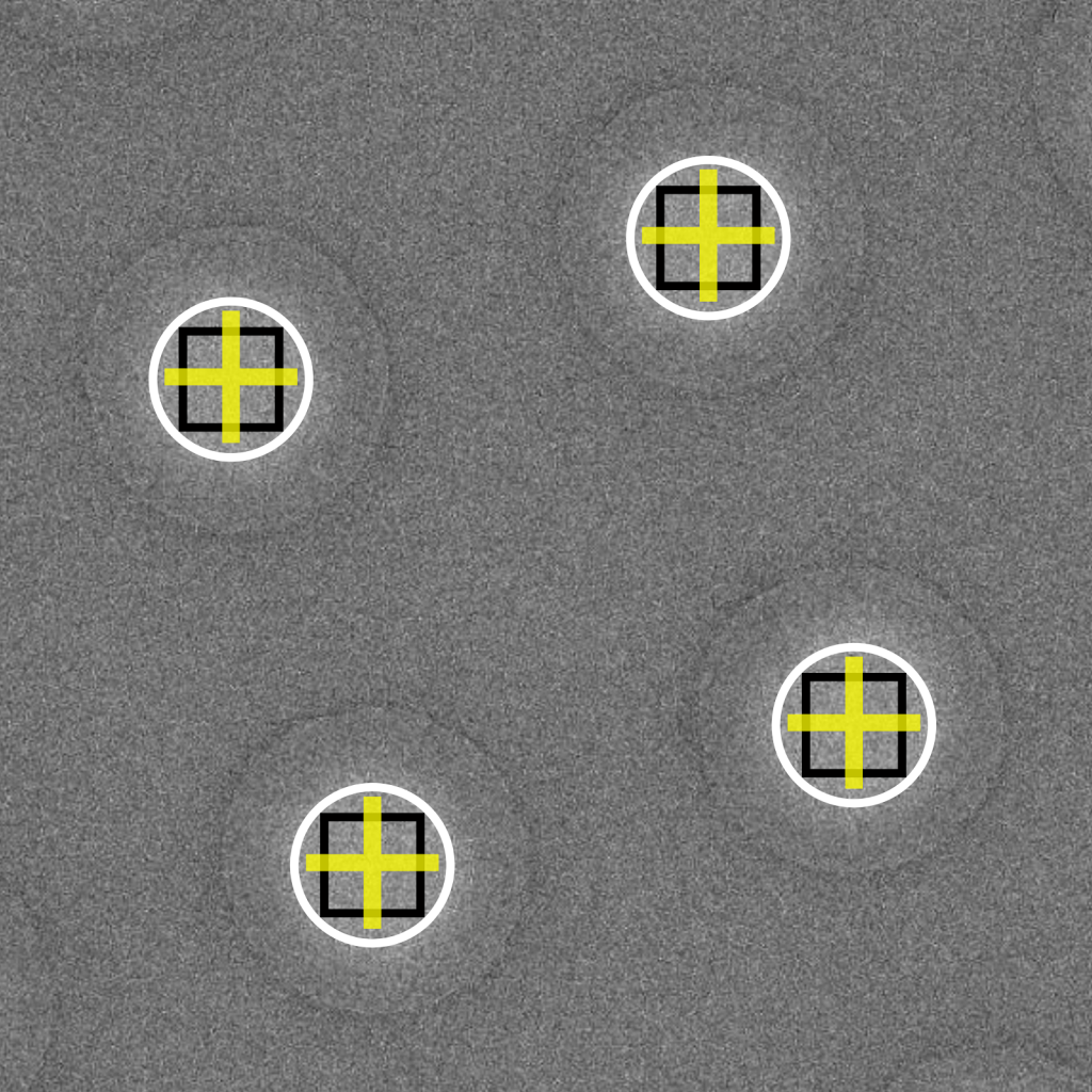
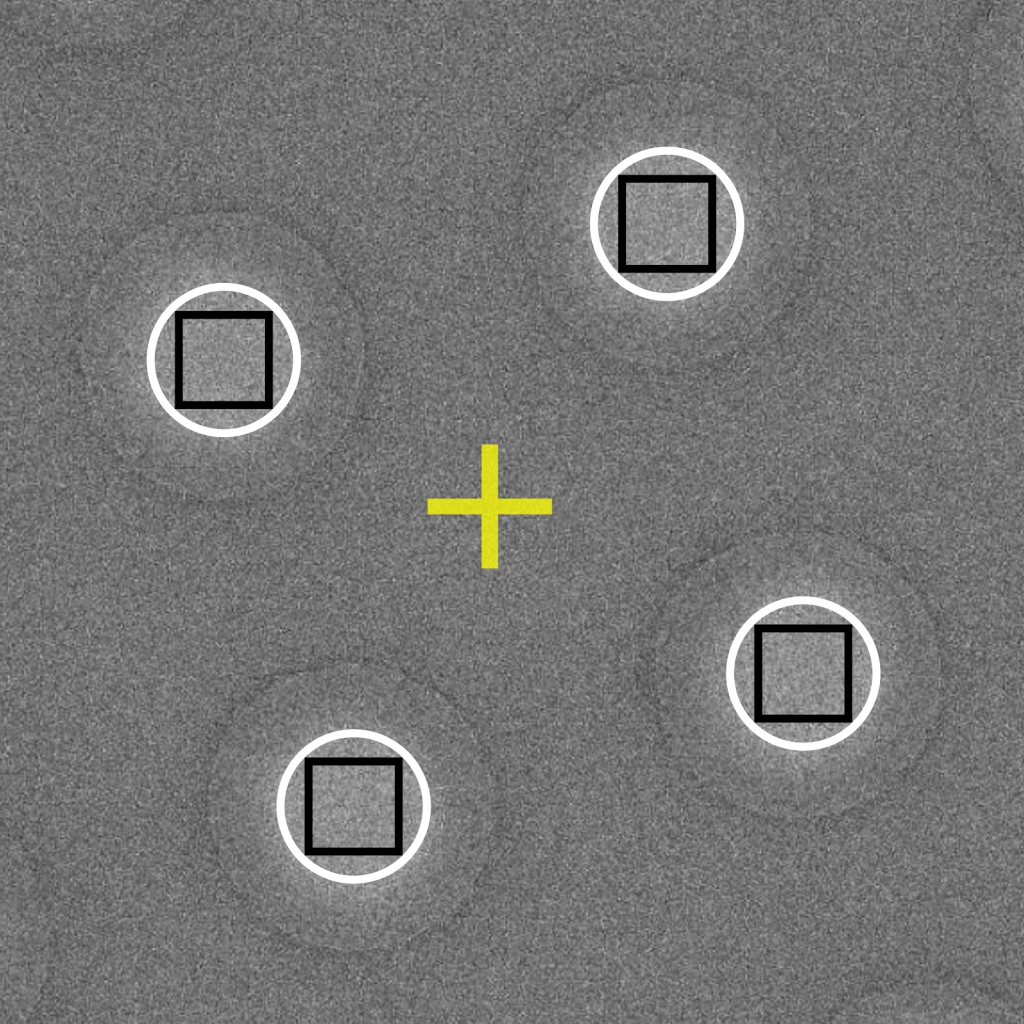
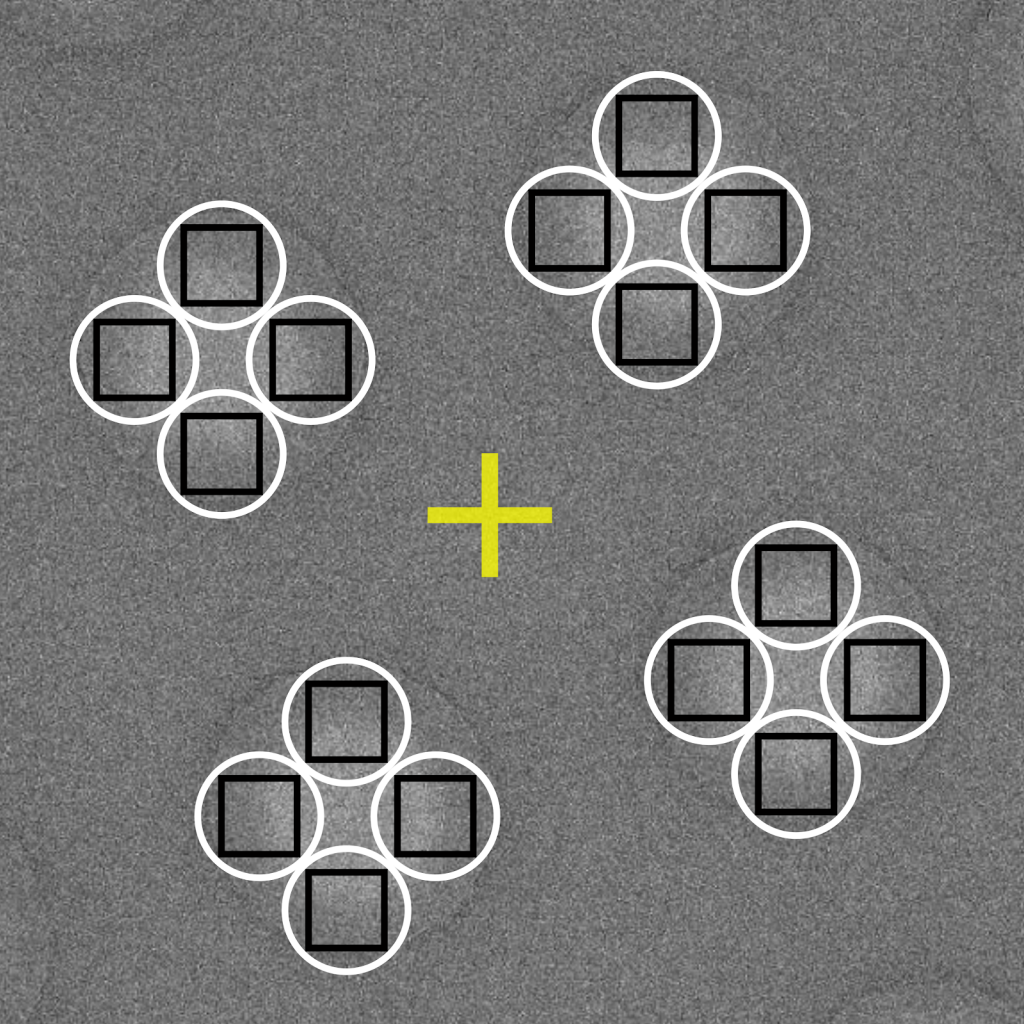
Different targeting strategies are possible depending on your microscope settings and resolution goals. A summary of various common options are available below. In each provided example, the yellow crosshair represents the search mode centering position, the white circle represents the illuminated area, and black square represents the area captured by the camera.
The most conventional method of hole targeting is to mechanically center the stage over each hole. A relaxation time after centering is needed to stabilize the stage before focusing and recording are performed. Image recording is performed directly over the centered area, after which the stage position is moved to the next hole. This data collection strategy generally produces 1,000-2,000 movies per 24-hour session.
Data collection efficiency is greatly boosted by recording several images per stage movement. In this scheme, the stage is centered over a single focusing area, after which a beam-image shift is applied to record images in surrounding holes. Theoretically, shifting the beam in this manner limits the achievable resolution because the electron path is diverted away from the optical axis and causes coma aberrations. In practice, however, many high-resolution structures in the 2.5-3 Å range have been attained using this targeting strategy even with shifts up to several microns away from the centered position. The advantage of substantially higher throughput using this strategy often justifies the concerns about its resolution-limiting effects. If the resolution needs to extend beyond 2.0 Å, then pristine, on-axis imaging should be performed using the conventional targeting method of acquiring one image per physical stage movement.
An extension to the multi-hole targeting approach described above can be applied to record several images per hole. The number of images per hole will be dependent on the microscope settings (i.e., illuminated area) and grid properties (i.e., hole diameter). Using high magnifications and large hole diameters will permit more exposures per hole. Care must be taken when using this aggressive strategy to ensure that exposed areas are kept separated. This strategy potentially enables dozens of images to be recorded per stage movement and can produce several thousands of movies per 24-hour session.
The optimal data collection session strives to maximize the amount of high-quality images recorded per unit time. The user decisions discussed in this chapter—magnification, defocus range, total electron exposure, and hole targeting strategy—will set expectations on achievable resolutions and influence how data is processed. For most projects, standard data collection parameters of a ~1Å pixel size, -1 to -2 micron defocus range, 40-60 electrons per Å2, and aggressive multi-shot targeting are routine and generally yield structures in the ~3 Å resolution range. Deviations to these standard settings may be explored depending on the needs of the project. For instance, achieving reconstructions surpassing 2 Å generally require exceptionally well-behaved particles that are recorded using smaller pixel sizes and single-shot targeting over thin ice. More challenging specimens may be limited by the nature of the particles than by data collection settings (e.g., due to small size or structural heterogeneity). In the next and final chapter of CryoEM 101, we will discuss the fundamentals of image processing and 3D reconstruction and the exciting advances in software that enable users to get the most out of their data.
© Copyright 2024